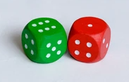
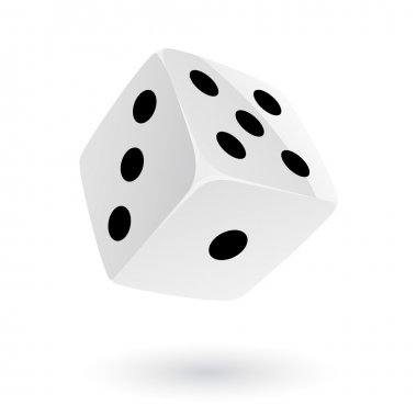
Lecture 9: Random Variables and Expectation

class: center, middle, inverse, title-slide

.title[
# Lecture 9: Random Variables and Expectation
]
.author[
### Robin Liu
]
.institute[
### UCSB
]
.date[
### 2022-07-06
]

---

class: inverse, middle, center
# Random variables
---
# Random variables
**"Definition"**: A *random variable* is a numerical outcome of our experiment.

Roll two dice and call the outcome of the green die `$X$` and the outcome
of the red die `$Y$`

Then `$X$` and `$Y$` are both random variables.

`$X+Y$`, `$XY$`, `$e^{\sin(XY)}$` are also random variables;
functions of r.v.s are r.v.s.

![](Lec8_files/twodice.png)
---
# Random variables

| rep 	|| X 	| Y 	| X + Y 	| X + Y == 6? 	|
|-----	||-----	|-------	|-----------	|---------------	|
| 1   	|| 4   	| 3     	| 7         	| FALSE         	|
| 2   	|| 4   	| 2     	| 6         	| TRUE          	|
| 3   	|| 1   	| 4     	| 5         	| FALSE         	|
| 4   	|| 2   	| 6     	| 8         	| FALSE         	|
| 5   	|| 6   	| 1     	| 7         	| FALSE         	|
---
# Random variables
Recall an **event** is a logical (TRUE or FALSE) outcome of an experiment.
Hence the expression `$X + Y = 6$` is an event.

Last time we found the probability of this event via simulation.

Notation: 
`\begin{align*}
\mathbb{P}(X + Y = 6) = \frac{5}{36}
\end{align*}`

--
Let's focus on the probabilities of a single dice roll,
the random variable `$X$`.

---
# Random variables
The randomness of a random variable is determined by its **probabilities**
which are governed by its **distribution**.

*Knowing the distribution means having complete information about the probabilities.*

Let `$X$` be the result of rolling a fair six-sided die.
What is the distribution of `$X$`?

![:scale 20%](Lec8_files/die.jpg)

We can write down the complete probabilistic behavior of `$X$` in a table.
This is the **distribution** of `$X$`.

| `$k$`      | 1 | 2 | 3 | 4 | 5 | 6 |
| ----------- | ----------- |----------- |----------- |----------- |----------- |----------- |
| `$\mathbb{P}(X = k)$`      | 1/6       |1/6       |1/6       |1/6       |1/6       |1/6       |

---
# Random variables
| `$k$`      | 1 | 2 | 3 | 4 | 5 | 6 |
| ----------- | ----------- |----------- |----------- |----------- |----------- |----------- |
| `$\mathbb{P}(X = k)$`      | 1/6       |1/6       |1/6       |1/6       |1/6       |1/6       |

Actually... is this all of the info? What is `$\mathbb{P}(X=7)$` or
`$\mathbb{P}(X = -\pi)$`?

Implicit in the table is that `$\mathbb{P}(X=k) = 0$` if `$k\neq 1, 2, \dotsc, 6$`.

We say the **support** of `$X$` is the set `$\{1, 2, \dotsc, 6\}$`;
it is the set of values with non-zero probabilities.
If the support is "discrete", we say `$X$` is a *discrete random variable*.

## Important
The sum of the probabilities must add up to 1.

---
# Named distributions
| `$k$`      | 1 | 2 | 3 | 4 | 5 | 6 |
| ----------- | ----------- |----------- |----------- |----------- |----------- |----------- |
| `$\mathbb{P}(X = k)$`      | 1/6       |1/6       |1/6       |1/6       |1/6       |1/6       |

Certain distributions are so common that we give them fancy names.
`$X$` follows *discrete uniform distribution on 1, 2, ..., 6*.

This is abbreviated `$X \sim \mathrm{DUnif}(\{1, 2, \dotsc, 6\})$`.

Let `$C = \{\text{cat, dog, fish, owl}\}$` and `$W \sim \mathrm{DUnif}(C)$`.

What is `$\mathbb{P}(W = \text{dog})$`?

The set `$C$` **parametrizes** the distribution.

Or: the distribution has **parameter** `$C$`, the set of possible outcomes.

---
# Bernoulli distribution

Consider an experiment of flipping a **biased** coin
and let `$X$` be the r.v. that *indicates* landing heads:

`$\begin{equation}X = \begin{cases}1 &\text{coin lands heads} \\ 0 & \text{coin lands tails}\end{cases}\end{equation}$`

If the coin lands heads with probability `$p$`, the distribution of `$X$`
can be written

| `$k$`      | 0 | 1 |
| ----------- | ----------- |----------- |
| `$\mathbb{P}(X = k)$`      | `$1-p$`       | `$p$`       |

`$X$` follows the *Bernoulli distribution with probability `$p$`*.

$$
X \sim \mathrm{Bern}(p)
$$
`$p$` is the **parameter** of the Bernoulli distribution.
It must satisfy `$0\leq p \leq 1$`.
---
# Bernoulli distribution
The distribution only concerns the probabilities of a random variable,
not the nature of the experiment

Let `$W$` indicate rolling an even number on a fair die.
What is the distribution of `$W$`?

A bag contains 10 black marbles, 1 red marble, and nothing else.
I choose a marble uniformly at random. 
Let `$Z$` indicate pulling out the red marble.
What is the distribution of `$Z$`?

I close my eyes and throw a dart at a map of the United States.
Let `$A$` indicate the dart landing on Alaska.
What is the distribution of `$A$`?

These are totally different experiments, but they are all Bernoulli r.v.s.
(with different probabilities).
---
# Binomial distribution
Consider flipping a biased coin `$n$` times.
Let `$p$` be the probability of landing heads.

Let `$X$` be the total number of heads in `$n$` tosses.

`$X$` is the *binomial distribution with `$n$` trials and probability `$p$`*
$$
X \sim \mathrm{Binom}(n, p)
$$

### Example
`$n = 2$`, `$p = 1/2$` leads to the possible outcomes (HH, HT, TH, TT)

| `$k$`      | 0 | 1 | 2 |
| ----------- | ----------- |----------- | ------|
| `$\mathbb{P}(X = k)$`      | `$1/4$`       | `$1/2$`       | `$1/4$` |

Note `$\mathrm{Bern}(p)$` is the same as `$\mathrm{Binom}(1, p)$`.

---
# Binomial distribution
### Four criteria for the binomial distribution
1. There is a **fixed** number of trials `$n$`.
2. Each trial is **not affected by** of the other trials (independence).
3. Each trial has two possible outcomes, `$0$` or `$1$`. We call an outcome of `$1$` a *success*.
4. The probability of success for each trial is `$p$`.

Then the total number of success, `$X$` is a binomial r.v. and we write
$$
X \sim \mathrm{Binom}(n, p).
$$

What is the support of `$X$`? Is `$X$` a discrete r.v.?

---
# Binomial distribution
For discrete r.v.s, `$\mathbb{P}(X = k)$` is the *probability mass function* or **pmf** of `$X$`.
It is a function of `$k$`.

The pdf of `$X$` if `$X\sim \mathrm{Binom}(n, p)$` is
$$
\mathbb{P}(X = k) = \binom{n}{k}p^k (1-p)^{n-k}\; \text{for `$k = 0, 1, \dotsc, n$`}
$$
--

Let `$X \sim \mathrm{Binom}(100, 1/3)$`. Determine `$\mathbb{P}(X = 40)$`.
--
.pull-left[

```r
n <- 100
p <- 1/3
k <- 40
```
`choose(n, k) \* p^k \* (1-p)^(n-k)`

```
## [1] 0.03075091
```
]
--
.pull-right[
Better way:

```r
dbinom(40, size = 100, prob = 1/3)
```

```
## [1] 0.03075091
```
]
---
# Binomial distribution
The ratio of the area of Alaska to the area of the United states is
about 0.18.

I throw 10 darts independently at random at the map. What is the probability
that exactly 4 of the darts land on Alaska?

What is the probability *less than or equal to* 4 darts land on Alaska?

`$\mathbb{P}(X \leq 4)$`.

<div class="countdown" id="timer_62c5a779" style="right:0;bottom:0;" data-warnwhen="0">
<code class="countdown-time"><span class="countdown-digits minutes">01</span><span class="countdown-digits colon">:</span><span class="countdown-digits seconds">00</span></code>
</div>
---
# Binomial distribution
What is the probability *less than or equal to* 4 darts land on Alaska?
`$X \sim \mathrm{Binom}(10, 0.18)$`.

Find `$\mathbb{P}(X \leq 4)$`:

```r
pbinom(4, size = 10, prob = 0.18)
```

```
## [1] 0.9786771
```

`dbinom` gives the pmf

```r
dbinom(4, size = 10, prob = 0.18)
```

```
## [1] 0.06701815
```

`pbinom` gives the *cumulative probabilities*, the *cdf*.

```r
pbinom(4, size = 10, prob = 0.18)
```

```
## [1] 0.9786771
```

---
# Binomial distribution
Let `$X \sim \mathrm{Binom}(10, 0.18)$`.

Find `$\mathbb{P}(X < 4)$`.
This is equivalent to
$$
\mathbb{P}(X =0) + \mathbb{P}(X = 1)+ \mathbb{P}(X =2)+\mathbb{P}(X =3)
$$
<div class="countdown" id="timer_62c5aa35" style="right:0;bottom:0;" data-warnwhen="0">
<code class="countdown-time"><span class="countdown-digits minutes">02</span><span class="countdown-digits colon">:</span><span class="countdown-digits seconds">00</span></code>
</div>

Find `$\mathbb{P}(X \geq 4)$`.
This is equivalent to 
$$
\mathbb{P}(X =4) + \mathbb{P}(X = 5)+ \dotsb + \mathbb{P}(X = 10)
$$
<div class="countdown" id="timer_62c5a7e2" style="right:0;bottom:0;" data-warnwhen="0">
<code class="countdown-time"><span class="countdown-digits minutes">02</span><span class="countdown-digits colon">:</span><span class="countdown-digits seconds">00</span></code>
</div>

---
# Binomial distribution
### Generating binomial observations
Let's actually throw the 10 darts at Alaska using R.

```r
sum(sample(0:1, 10, replace = T, prob = c(0.82, 0.18)))
```

```
## [1] 3
```

Easier way:

```r
rbinom(1, size = 10, prob = 0.18)
```

```
## [1] 1
```

We can generate multiple observations of this experiment.

```r
rbinom(5, size = 10, prob = 0.18)
```

```
## [1] 0 0 2 4 2
```

How many darts did we throw in total?

**Important:** The first argument to `rbinom` is the number of observations
of the experiment. The `size` is the number of trials in each observation.

---
# Binomial distribution expectation
Remember a r.v. is the numerical outcome of a random experiment.
The **expectation** of a random variable is the long-run average of this outcome
as we do `$n\to\infty$` replications of the experiment.

$$
\lim_{n\to\infty} \frac{x_1 + x_2 + \dotsc + x_n}{n}.
$$

Let `$X$` be the r.v. that indicates the number heads after flipping a fair
coin `$n=10$` times.

$$ X \sim \mathrm{Binom}(10, 1/2)$$

Estimate the expectation through directly simulating `$10,000$` replications

---
# Binomial distribution expectation
Easy way using `rbinom`:

```r
mean(rbinom(10000, size = 10, prob = 0.5))
```

```
## [1] 5.0052
```

Built-in functions are **very** useful!

---
# Distributions in R
R comes with many named distributions built in.

The functions below illustrate a pattern in R:
- `dbinom(x, size, prob)`
- `pbinom(q, size, prob)`
- `rbinom(n, size, prob)`

Suppose `$Y\sim \mathrm{booga}(\text{params})$` (not a real distribution). Then
- `dbooga(x, params)` evaluates the pmf (or pdf) of `booga` at `$x$`
- `pbooga(q, params)` gives the *cumulative* probabilities: `$\mathbb{P}(Y \leq q)$`
- `rbooga(n, params)` generates `$n$` observations of `$Y$`. Also called **random variates**.

We will soon see 
- `dunif`, `punif`, `runif`
- `dnorm`, `pnorm`, `rnorm`