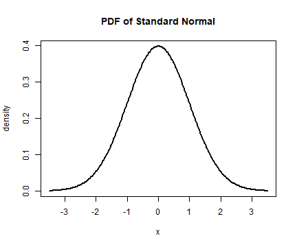
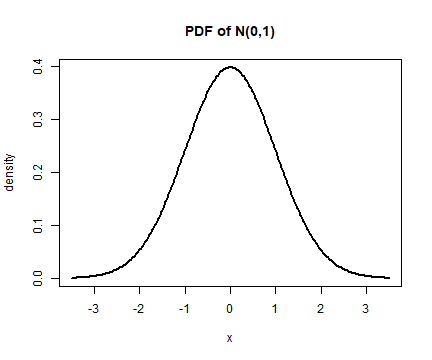
Lecture 10: Continuous Random Variables

class: center, middle, inverse, title-slide

.title[
# Lecture 10: Continuous Random Variables
]
.author[
### Robin Liu
]
.institute[
### UCSB
]
.date[
### 2022-07-08
]

---

# Random variables
Recall that
a *random variable* is a numerical outcome of an experiment.

Last time we looked at *discrete random variables*.
`$X$` is *discrete* if its support is a discrete set.

**Discrete sets:**
- `$\{0, 1, 2, \dotsc, n\}$`
- `$\mathbb{N} = \{1, 2, 3, \dotsc\}$`
- `$\mathbb{Z} = \{\dotsc, -1, 0, 1, \dotsc\}$`
- `$\{\text{dog}, \text{cat}, \text{fish}\}$`
- The set of all animals in existence.

**Continuous sets:**
- `$[0,1] = \{x: 0\leq x\leq 1\}$`
- `$(-12,67] = \{x: -12< x\leq 67\}$`
- `$\mathbb{R} = (-\infty, \infty)$`
- The waiting time for a bus at North Hall.

---
# Continuous Random Variables
Suppose a bus arrives every 10 minutes.
You arrival at the bus stop at a random time.
How long will you have to wait?

Let `$X$` be the time you must wait for the next bus.

`$X$` is a continuous r.v. with support `$(0,10)$`.

What is the **distribution** of `$X$`? This depends on some assumptions.
---
# Uniform distribution
Suppose you are equally likely to arrive at any time.
Draw pic

A plot of the "likelihood" might look like this:
<img src="Lec10_files/figure-html/unnamed-chunk-2-1.png" style="display: block; margin: auto;" />

---
# Uniform distribution
What we have plotted is the *probability density function (pdf)*
of the **uniform distribution**.

Write `$X \sim \mathrm{Unif}(0, 10)$`.
The parameters specify the lower and upper bound of the support.
<img src="Lec10_files/figure-html/unnamed-chunk-3-1.png" style="display: block; margin: auto;" />

---
# Uniform distribution
<img src="Lec10_files/figure-html/unnamed-chunk-4-1.png" style="display: block; margin: auto;" />

Unlike discrete r.v.s, **the y-axis does not give probabilities**.

The y-axis is the **density**, not the *mass* (p**d**f vs p**m**f).

---
# Uniform distribution
The builtin R functions are `dunif`, `punif`, and `runif`.
By default, `runif` generates observations from `$\mathrm{Unif}(0,1)$`:

```r
runif(5)
```

```
## [1] 0.37219838 0.04382482 0.70968402 0.65769040 0.24985572
```

Generate waiting times for `$X \sim \mathrm{Binom}(0, 10)$`:

```r
runif(5, min = 0, max = 10)
```

```
## [1] 3.000548 5.848666 3.334671 6.220120 5.458286
```

---
# Uniform distribution
`dunif` gives the **values of the density function**.
<img src="Lec10_files/figure-html/unnamed-chunk-7-1.png" style="display: block; margin: auto;" />

```r
dunif(4, min = 0, max = 10)
```

```
## [1] 0.1
```

## ACHTUNG!
This **does not** say `$\mathbb{P}(X = 4)= 0.1$`.

---
# Uniform distribution
### Computing probabilities
<img src="Lec10_files/figure-html/unnamed-chunk-9-1.png" style="display: block; margin: auto;" />

Note that the **area under the curve** equals 1.

Unlike discrete r.v.s, for continuous r.v.s we must compute
the area under curve to find the probabilities.

What is `$\mathbb{P}(X \leq 4)$`?

---
# Uniform distribution
<img src="Lec10_files/figure-html/unnamed-chunk-10-1.png" style="display: block; margin: auto;" />

`$\text{area of shaded region} = 0.10 \times 4 = 0.4$`

Hence: `$\mathbb{P}(X \leq 4) = 0.4$`

---
# Uniform distribution
Compute `$\mathbb{P}(2.5 \leq X \leq 4.3)$`.

`$$\mathbb{P}(2.5 \leq X \leq 4.3) = \text{area of shaded region} = 0.10 \times (4.3-2.5) = 0.18$$`

---
# Uniform distribution
Compute `$\mathbb{P}(2.5 \leq X \leq 4.3\; \textbf{OR}\; X > 8)$`.

`$\text{area of shaded region} = 0.10 \times (4.3-2.5) + 0.10 \times (10 -8)= 0.38$`

Since the total area under the curve equals `$1$`, all probabilities
are between `$0$` and `$1$`, which is good.

---
# Uniform distribution
<img src="Lec10_files/figure-html/unnamed-chunk-13-1.png" style="display: block; margin: auto;" />
Recall that *cumulative probabilities* are of the form `$\mathbb{P}(X \leq k)$`.

`punif` gives the cumulative probabilities.

```r
punif(4, min = 0, max = 10)
```

```
## [1] 0.4
```

---
# Uniform distribution
Compute `$\mathbb{P}(2.5 \leq X \leq 4.3)$` using `punif`.

```r
punif(4.3, min = 0, max = 10) - punif(2.5, min = 0, max = 10)
```

```
## [1] 0.18
```

---
# Uniform distribution
Compute `$\mathbb{P}(2.5 \leq X \leq 4.3\; \textbf{OR}\; X > 8)$` with `punif`.

<div class="countdown" id="timer_62c88b4f" style="right:0;bottom:0;" data-warnwhen="0">
<code class="countdown-time"><span class="countdown-digits minutes">02</span><span class="countdown-digits colon">:</span><span class="countdown-digits seconds">00</span></code>
</div>
---
# Uniform distribution
So what is `$\mathbb{P}(X = 4)$`?
<img src="Lec10_files/figure-html/unnamed-chunk-18-1.png" style="display: block; margin: auto;" />

Probabilities are areas under the curve.
But the "area under" the curve at the point 4 is a one-dimensional line
with no area.

*The probability a continuous r.v. takes on a single point is ZERO*.

What does this say about `$\mathbb{P}(X \leq 4)$` vs. 
`$\mathbb{P}(X < 4)$`?

---
# Normal distribution
The *most important* distribution.

Many continuous r.v.s are (approximately) normally distributed:
  - heights of people
  - weights of similar animals
  - measurements of items produced in a factory
  
![](Lec10_files/figure-html/unnamed-chunk-19-1.png)
---
# Normal distribution
The normal distribution has two parameters:
- the **mean** `$\mu$`
- the **standard deviation** `$\sigma$`

Write `$X\sim N(\mu, \sigma)$`.

`$N(0, 1)$` is called the **standard normal**.

![](Lec10_files/figure-html/unnamed-chunk-20-1.png)

---
# Normal distribution
<img src="Lec10_files/figure-html/unnamed-chunk-21-1.png" style="display: block; margin: auto;" />

---
# Normal distribution
<img src="Lec10_files/figure-html/unnamed-chunk-22-1.png" style="display: block; margin: auto;" />

---
# Normal distribution
In R

**binomial distribution** `$\mathrm{Binom}(\text{size},\, \text{prob})$`
- `dbinom(x, size, prob)`
- `pbinom(q, size, prob)`
- `rbinom(n, size, prob)`

**uniform distribution** `$\mathrm{Unif}(\text{min},\, \text{max})$`
- `dunif(x, min, max)`
- `punif(q, min, max)`
- `runif(n, min, max)`

Can you guess the functions for the normal distribution?

**normal distribution** `$N(\text{mean},\, \text{sd})$`
- `dnorm(x, mean, sd)`
- `pnorm(q, mean, sd)`
- `rnorm(n, mean, sd)`

---
# Normal distribution
<img src="Lec10_files/figure-html/unnamed-chunk-23-1.png" style="display: block; margin: auto;" />

```r
dnorm(2, mean = 1, sd = 1.5)
```

```
## [1] 0.2129653
```

`dnorm` gives the *values of the normal pdf*

---
# Normal distribution
<img src="Lec10_files/figure-html/unnamed-chunk-25-1.png" style="display: block; margin: auto;" />

```r
pnorm(2, mean = 1, sd = 1.5)
```

```
## [1] 0.7475075
```

`pnorm` gives the *cdf* `$\;\mathbb{P}(X \leq 2)$`

---
# Normal distribution
<img src="Lec10_files/figure-html/unnamed-chunk-27-1.png" style="display: block; margin: auto;" />

```r
set.seed(101)
rnorm(10, mean = 1, sd = 1.5)
```

```
##  [1]  0.51094526  1.82869278 -0.01241577  1.32153919  1.46615383  2.76094943
##  [7]  1.92818478  0.83089853  2.37554243  0.66511095
```
`rnorm` generates normal random variates (or observations)

---
# Normal distribution
Let `$X \sim N(1, 1.5)$`.
Compute `$\;\mathbb{P}(-1.25 < X \leq 2)$`

<img src="Lec10_files/figure-html/unnamed-chunk-29-1.png" style="display: block; margin: auto;" />
--

## Method 1: Solve
$$
\int_{-1.25}^{2} \frac{1}{1.5\,\sqrt{2\pi}}e^{-\frac{1}{2}\left(\frac{x - 1}{1.5}\right)^2}\mathrm{d}x
$$
--

---
# Normal distribution
Let `$X \sim N(1, 1.5)$`.
Compute `$\;\mathbb{P}(-1.25 < X \leq 2)$`

## Method 2: `pnorm`

```r
pnorm(2, mean = 1, sd = 1.5) - pnorm(-1.25, mean = 1, sd = 1.5)
```

```
## [1] 0.6807003
```

---
# Normal distribution
Let `$X \sim N(1, 1.5)$`.
Compute `$\;\mathbb{P}(X \geq 2)$`

---
# Assessing normality
### Is our data normally distributed?
A visual way to check this is by using a *Q-Q plot* (quantile-quantile plot).
The points should lie along the line.

```r
qqnorm(iris$Sepal.Width)
qqline(iris$Sepal.Width, col = "red")
```

---
# Assessing normality
### Is our data normally distributed?

```r
qqnorm(iris$Petal.Length)
qqline(iris$Petal.Length, col = "red")
```

This is a visual, heuristic way to check normality, but sometimes its the best we've got.