CMA-ES
Comparing the performance of two blackbox or "derivative-free" optimization methods.
We discuss the Covariance Matrix Adaptation Evolution Strategy (CMA-ES), a blackbox optimization algorithm for arbitrary functions that are not necessarily smooth or convex. We compare the performance of CMA-ES against a more naive approach on a couple of test functions, demonstrating that the clever updating strategies in CMA-ES result in better performance. Finally, we look at an application of CMA-ES in real research related to image-guided navigation during surgery. A comprehensive guide to CMA-ES is provided in [1]. All code, including the implementation and code to generate the plots in this report, are on Github.
\(\renewcommand{\vec}[1]{\boldsymbol{\mathbf{#1}}} \newcommand{\R}{\mathbb{R}} \newcommand{\EE}{\mathbb{E}}\)
1 Introduction
When a function is smooth and convex, we can find the global minimizer using first-order methods such as gradient descent. Moreover, the theoretical properties of the update steps are well understood, e.g. we can give an upper bound on the step size that guarantees convergence, or use backtracking to find a suitable reduction of the objective function at each step.
Minimization problems are much harder when the objective function is non-smooth. If a function is not differentiable, we certainly cannot perform gradient descent. If a function is not convex, we cannot conclude that a local minimum we have found is a global minimum. Despite these challenges, there exist methods that aim to minimize non-smooth and non-convex functions. Such methods are called blackbox or derivative-free methods, indicating that evaluating the derivative is not necessary.
Our setting is the simple unconstrained problem given by
\[\operatorname*{minimize}_{\vec x \in \R^n} f(x),\quad f\colon \mathbb{R}^n \to\mathbb{R} \text{ is an arbitrary function.}\]We require that \(f\) can be evaluated at every point in \(\mathbb{R}^n\). We compare two methods for this problem: the cross-entropy method and the Covariance Matrix Adaptation Evolution Strategy (CMA-ES). Both of these methods place a probability distribution, called the proposal distribution, over the domain of \(f\) and at each iteration, sample points from the domain and update the distribution based on a subset of elite design points. The mean of the ultimate distribution at convergence yields an estimate for the minimizer. In this project we use the multivariate normal proposal distribution for both methods.
We first give an outline of the cross-entropy method, focusing on how it performs parameter updates using maximum likelihood estimates. Then we explore the CMA-ES parameter update steps. We compare the performance of the two methods on the 2-dimensional flower function and the 20-dimensional Michalewicz function, given in Appendix A.2.
2 A Naive Approach
2.1 MLEs and Cross-entropy
We wish to minimize \(f\), but aside from its value at points in the domain, we know nothing of the structure of \(f\). Our strategy is to sample points in the domain via a \(N(\vec\mu, \vec \Sigma)\) distribution and update \(\vec \mu\) and \(\vec \Sigma\) based on a subset of “elite” sample points, i.e. those with low \(f\) value. We call this approach “naive” because \(\vec \mu\) and \(\vec \Sigma\) are updated in the most obvious way: they become the MLEs of the elite sample.
This is Algorithm 1. Convergence can be taken to mean that the mean vector of the distribution has not changed beyond a provided tolerance. In the final two steps we update \(\vec \mu'\) to be the sample average of the elite sample and \(\vec \Sigma'\) to be the sample covariance of the elite sample, with respect to \(\vec \mu'\).
The algorithm is intuitively appealing. In fact, it can be shown that this algorithm is an instance of the cross-entropy method for multivariate normals; in this case, minimizing the cross-entropy of the two distributions amounts to computing the MLE.
Algorithm 1: Cross-entropy with Multivariate Gaussian (CEMVN)
Require: \(f\colon \R^n \to \R\), initial parameters \((\vec \mu^{(0)}, \vec\Sigma^{(0)})\), \(m\) size of sample, \(m_{\text{elite}}\) size of elite subsample.
Ensure: \(\vec \mu^{(T)}\) is the mean of the final distribution and the proposed minimizer.
For \(t = 0, 1, \dotsc\) until convergence:
- Sample points \(\vec x_1, \dotsc, \vec x_m\) from distribution \(N(\vec\mu^{(t)}, \vec \Sigma^{(t)})\).
- Let \(\vec x_{(1)}, \ldots, \vec x_{(m)}\) be the sample ordered so that \(f(\vec x_{(j)}) \leq f(\vec x_{(j+1)})\).
- Update \(\vec \mu^{(t+1)} \leftarrow \text{mean}(\vec x_{(1)}, \ldots, \vec x_{(m_{\text{elite}})})\)
- Update \(\vec \Sigma^{(t+1)} \leftarrow \frac{1}{m_{\text{elite}}}\sum_{k=1}^{m_{\text{elite}}} (\vec x^{(k)} - \vec\mu^{(t+1)})(\vec x^{(k)} - \vec\mu^{(t+1)})^\intercal\)
2.2 Issues with the naive approach
We motivate the CMA-ES approach in the next section by outlining three problems with the naive method.
- In updating the mean, the elite points are equally weighted. The sample average of the elite points are calculated without regard to their values of \(f\).
- In updating the covariance matrix, the update path is not remembered.
- The lack of scaling parameter means the covariance matrix may prematurely shrink.
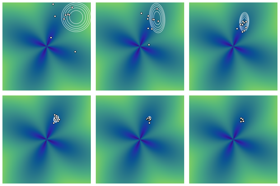
These problems are highlighted in the Figure 1. We ran CEMVN on the flower function, initialized with a mean of \((2,2)\) and identity covariance. Blue and green indicates smaller and larger values of the flower function, respectively. The function is minimized near the center of the “flower”, which is at the origin. Each plot shows the ten elite points sampled from the bivariate normal whose level curves are also plotted in white. While the mean starts to shift toward the origin, the covariance degenerates too quickly for enough points to be sampled near the optimum, resulting in premature convergence.
3 The Covariance Matrix Adaptation Evolutionary Strategy
The CMA-ES method remedies these issues. At each step, \(\vec x \sim N(\vec \mu, \sigma^2 \vec\Sigma)\) is sampled. The following summarizes the key differences from the naive approach.
- The mean vector is updated by a weighted average of the elite points.
- The covariance matrix is updated by considering the elite sample points along with correlations between previous generations. This is accomplished via cumulation.
- The step size is controlled via the parameter \(\sigma\), which is also updated in a data-adaptive way via cumulation. This ameliorates premature convergence.
The last two points cause the covariance matrix to adapt to the samples, unlike the cross-entropy method in which previous information is discarded. Like the cross-entropy method, we use \(m\) samples at each step and select an elite sample of size \(m_{\text{elite}}\). The function \(f\colon \R^n \to \R\) is to be minimized. We will discuss how the method updates the mean, covariance matrix, and overall step size parameters. These update steps form the basis of full algorithm, given in Appendix A.3.
3.1 Updating the mean
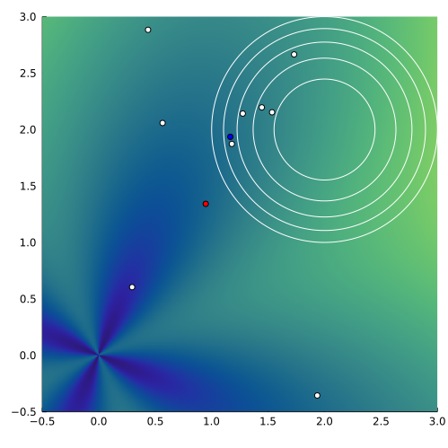
Unlike the naive method, the mean is updated by weighting each elite point according to its \(f\) value. Let \(\vec x_{(1)}, \ldots, \vec x_{(m_{\text{elite}})}\) be the elite sample such that \(f(\vec x_{(i)}) \leq f(\vec x_{(i+1)})\). The mean is updated as \begin{equation} \label{eq:meanstep} \vec\mu’ = \sum_{i=1}^{m_{\text{elite}}} w_i \vec x_{(i)}, \quad w_i = \log \frac{m+1}{2} - \log i\; \text{for $i = 1,\ldots, m_{\text{elite}}$}. \end{equation} These values of weights \(\{w_i\}\) are recommended by the authors of the original work; they are decreasing, hence heavier for the \(x_{(i)}\) where \(i\) is small. A comparison of the weighted versus the unweighted (naive) mean updated is shown in Figure 2. Due to the weights, the new mean is more aggressively pulled toward the origin.
The weights \(w_i\) are characterized by its variance effective selection mass, given by
\[\mu_{\text{eff}} = \frac{1}{\sum_{i=1}^{m_{\text{elite}}} w_i^2}.\]This value will show up in the sequel as a part of the recommended settings for various parameters of the algorithm.
3.2 Updating the covariance matrix
Unlike the naive method in which covariance information from previous generations is discarded, CMA-ES leverages information from the entire population as well as correlations between successive generations. The final update in (\ref{eq:covupdate}) accomplishes this with three terms: the previous covariance matrix, a rank-one update, and a rank-\(\mu\) update. We describe these in turn.
3.2.1 The Rank-\(\mu\) update
Consider again the covariance updating step in Algorithm 1:
\[\vec \Sigma^{(t+1)} \gets\frac{1}{m_{\text{elite}}}\sum_{k=1}^{m_{\text{elite}}} (\vec x^{(k)} - \vec\mu^{(t+1)})(\vec x^{(k)} - \vec\mu^{(t+1)})^\intercal.\]Since \(\vec\mu^{(t+1)}\) is the sample mean, this expression is the variance within the sampled points \(\vec x^{(k)}\). Instead, the expression
\[\frac{1}{m_{\text{elite}}}\sum_{k=1}^{m_{\text{elite}}} (\vec x^{(k)} - \vec\mu^{(t)})(\vec x^{(k)} - \vec\mu^{(t)})^\intercal\]where \(\vec\mu^{(t+1)}\) is replaced by \(\vec\mu^{(t)}\), the mean of the original distribution, describes the variance of the sampled steps. As in the mean update, we give a heavier weight to more “successful” steps using the weights \(w_i\) by defining
\[\vec\Sigma_{\mu}^{(t)} = \sum_{k=1}^{m_{\text{elite}}} w_i (\vec x^{(k)} - \vec\mu^{(t)})(\vec x^{(k)} - \vec\mu^{(t)})^\intercal.\]Sampling from the covariance matrix \(\vec\Sigma_{\mu}^{(t)}\) tends to reproduce the steps resulting in large decrease of $f$.
To finish up the rank-\(\mu\) update, we scale \(\vec\Sigma_{\mu}^{(t)}\) by the step size parameter \(\sigma^{(t)}\) (see Sec 3.3) so that these matrices are comparable across different generations, and then we ``smooth’’ the result across different generations. The final covariance matrix \(\vec\Sigma^{(t)}\) is updated as follows:
\[\vec\Sigma^{(t+1)} = \left(1 - c_\mu \sum_{i=1}^{m_{\text{elite}}} w_i\right) \vec\Sigma^{(t)} + c_\mu \frac{1}{\sigma^{(t)^2}} \vec\Sigma_\mu^{(t)}.\]The constant \(0\leq c_\mu \leq 1\) is a learning rate which controls how much information from previous generations is kept. Several of these tuning parameters appear in the sequel. They are \(c_\mu, c_c, c_1, c_\sigma\), and \(d_\sigma\). Their recommended values are given in Appendix A.1.
This update is called “rank-\(\mu\)” because it can be shown that the outer product in \(\vec\Sigma_\mu^{(t)}\) has rank \(\min(\mu, n)\).
3.2.2 The Rank-one update
While the rank-\(\mu\) update estimates the covariance matrix from all the steps in a single generation, we would also like to consider the evolution of steps throughout the previous generations. To this end, define the evolution path as the sequence of steps (the mean updates) taken by the algorithm normalized by the factor \(\sigma^{(t)}\) at each step. For example, the evolution path of the first three steps is
\[\frac{\vec\mu^{(3)} - \vec\mu^{(2)}}{\sigma^{(2)}} +\frac{\vec\mu^{(2)} - \vec\mu^{(1)}}{\sigma^{(1)}} +\frac{\vec\mu^{(1)} - \vec\mu^{(0)}}{\sigma^{(0)}}.\]The evolution path is actually constructed as a cumulation using a smoothing parameter \(c_c\) and is given by \begin{equation} \label{eq:cum} \vec p_c^{(t+1)} = (1-c_c)\vec p_c^{(t)} + \sqrt{c_c (2-c_c)\mu_{\text{eff}}} \frac{\vec\mu^{(t+1)} - \vec\mu^{(t)}}{\sigma^{(t)}}, \end{equation}
Finally, a parameter \(c_1\) controls the learning rate for this update and the final rank-one update is
\[\vec\Sigma^{(t+1)} = (1-c_1)\vec\Sigma^{(t)} + c_1 \vec p_c^{(t+1)}\vec p_c^{(t+1)^\intercal}.\]In this way, information about the successive steps between generations is used in updating the covariance matrix.
3.2.3 Putting it all together
Putting together both updates, we get the final covariance matrix update
\begin{equation} \label{eq:covupdate} \vec \Sigma^{(t+1)} =\left(1-c_1-c_\mu \sum_{i=1}^{m_{\text{elite}}} w_i\right)\vec \Sigma^{(t)} + c_1 \vec p_c^{(t+1)} \vec p_c^{(t+1)^\intercal} + c_\mu \frac{1}{\sigma^{(t)^2}} \vec\Sigma_{\mu}^{(t)}. \end{equation}
The update combines all the steps in a single generation with the overall step between all generations. The term \(-c_1 - c_\mu \sum_{i=1}^{m_{\text{elite}}} w_i\) is typically close to or equal to zero.
3.3 Updating the step size
Although the covariance matrix update allows the shape of the multivariate normal distribution to evolve, it is necessary for performance to control the overall scale of the distribution. This is done by the parameter \(\sigma^{(t)}\) at each step.
To update \(\sigma^{(t)}\), we keep track of the evolution path using cumulation as in \((\ref{eq:cum})\), except we normalize each step by pre-multiplying by \(\vec\Sigma^{(t)^{-1/2}}\), which has the effect of normalizing the step vector. Starting with \(\vec p_\sigma^{(0)}\), the path is updated by
\[\vec p_\sigma^{(t+1)} = (1-c_\sigma)\vec p_\sigma^{(t)} + \sqrt{c_\sigma(2-c_\sigma)\mu_{\text{eff}}}\; \vec \Sigma^{(t)^{-1/2}}\; \frac{\vec \mu^{(t+1)} - \vec \mu^{(t)}}{\sigma^{(t)}}.\]where \(c_\sigma\) controls the learning rate.
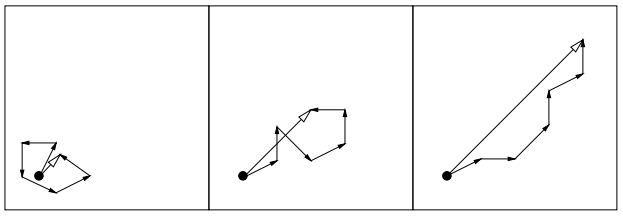
The key idea of the step size update is to increase the step size if the length of normalized steps exceed the expected length of a \(N(\vec 0, \vec I)\) vector, and decrease the step size if the length is less than what is expected from a \(N(\vec 0, \vec I)\) vector. This is depicted in Figure 3, which is copied from [1]. Let \(\vec Z \sim N(0, \vec I)\) be a standard normal random vector. When the individual step sizes in the evolution path are uncorrelated, the length of the normalized evolution path should approximate \(\EE \lVert{\vec Z}\rVert_2 \approx \sqrt{n} + O(1/n)\). If the individual step sizes in the evolution path are positively correlated, the overall evolution path length exceeds \(\EE \lVert{\vec Z}\rVert_2\) and the step size should be increased to take advantage of the correlation. Finally, if the individual step sizes are negatively correlated, the length of the evolution path is smaller than expected random length, and the step size should be decreased to explore the local area. All of this is accomplished by looking at the ratio \(\lVert{\vec p_\sigma^{(t+1)}}\rVert_2 / \EE \lVert{\vec Z}\rVert_2\).
The step size is updated by \begin{equation} \label{eq:stepupdate} \sigma^{(t+1)} = \sigma^{(t)} \exp\left(\frac{c_\sigma}{d_\sigma} \left(\frac{\lVert{\vec p_\sigma^{(t+1)}}\rVert_2 }{ \EE \lVert{\vec Z}\rVert_2} - 1\right)\right). \end{equation} where \(d_\sigma\) is a step size adaptation parameter. In this way, the step size adapts to the evolution path, stretching and shrinking the overall scale depending on the length of \(\vec p_\sigma^{(t+1)}\) relative to the expected length of \(\vec Z\).
3.4 Performance on the flower function
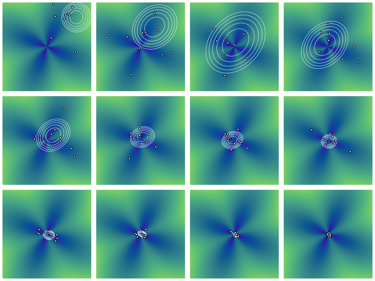
Figure 4 shows the result of running CMA-ES on the flower function with the same initial configuration as in Section 2.2. We see the adaptation in action: the variances are scaled larger at the start and prevent premature convergence. Compare this behavior to that of Figure 1.
3.5 Performance on the Michalewicz function
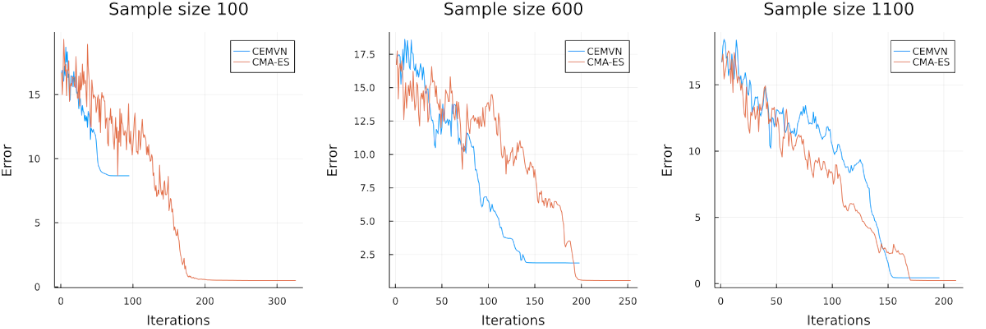
In this section, we examine the performance of CMA-ES against that of the cross-entropy method on a higher-dimensional function. We use the Michalewicz function given in Appendix A.2 with dimension \(d= 20\), where it is known that the function has \(20!\) local minima and that that the minimum is approximately \(-19.637\) [2]. Due to the higher dimensionality, we require more samples at each stage for both methods. We ran our implementations of CMA-ES and CEMVN (cross-entropy with multivariate normal) using sample sizes of 100, 600, and 1100 initialized at the point \((1, \dotsc, 1) \in \R^{20}\).
4 Application to spinal imaging
We turn to [3], which compares CMA-ES to other competing methods on the problem of registering images in the course of spinal surgery. Image-guided navigation is a surgical technique whereby a navigation system maps in real time the location of a surgeon’s instruments on a subject to a computerized image of the subject, such as a preoperative CT scan. Here is a short video explanation of how it works. During surgery, a calibration step is necessary so that the position of the instrument on the patient matches the graphic position of the instrument on the image. This important step is called registration. If a CT scan were improperly registered, the surgeon would see a digital representation of his instrument in the different location compared to where it actually is on the patient: this can be disastrous.
In the course of spinal surgery, additional imaging may be required for planning and the new images must be registered. One way to do this is to perform additional CT scans during surgery. Images from a CT scan have high resolution and can be easily registered with the preoperative image. However, this approach is invasive and exposes the subject to unnecessary radiation. An alternative method is to use ultrasounds, which are non-invasive; yet ultrasounds have a low signal-to-noise ratio so that registration is much more challenging.
The researchers in [3] consider registering noisy ultrasound images in the course of an operation. Surface points of the spine are extracted from a preoperative CT scan. The problem is to transform an intraoperative ultrasound image so that it is aligned with the surface points. This gives rise to the following optimization problem:
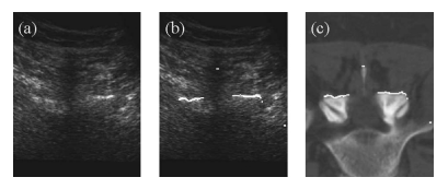
\[\operatorname*{maximize}_{\alpha, \beta, \gamma, \Delta_x, \Delta_y, \Delta_z} \sum_{i=1}^N u\left(R_{\alpha\beta\gamma}\cdot p_i + (\Delta_x, \Delta_y, \Delta_z)^\intercal\right)\]where \(R_{\alpha\beta\gamma}\) is a 3D rotation parametrized by the angles \(\alpha, \beta\) and \(\gamma\); \((\Delta_x, \Delta_y, \Delta_z)^\intercal\) is a vector representation of a translation in space; and \(p_i\) are points on the bone surface from the preoperative CT scan. The function \(u\) gives the “gray values” at various points on the ultrasound, where larger values indicate bright areas (bone) and smaller values indicate darker areas (tissue). The above objective function searches for rigid transformation parameters so that the bone surface from the preoperative CT scan best matches the bone from the ultrasound. Figure 6 from the paper shows an ideal registration of an ultrasound.
Since no additional structure is assumed in \(u\), CMA-ES is a good candidate for this problem, with suitable adjustments to make it a maximization algorithm.
The authors simulate randomly perturbed ultrasound images, run CMA-ES along with other methods on these images, and assess the performance of the resulting transformation parameters. The competing methods are gradient-based, where the gradient is estimated numerically. Figure 7 from their paper shows the results.
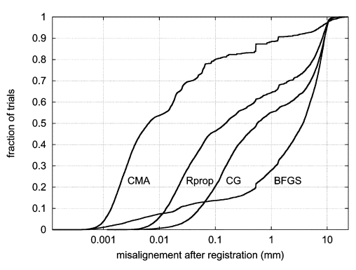
We see that CMA-ES outperforms the other methods by having a smaller degree of misalignment in a higher number of trials.
Appendix
A.1 Choice of tuning parameters
Throughout Section [3], we introduced various tuning parameters that affect the covariance matrix and step size update. In this section, we provide the recommended settings for these parameters. These settings are discussed in [1]. Recall that the variance effective selection mass is given by
\[\mu_{\text{eff}} = \frac{1}{\sum_{i=1}^{m_{\text{elite}}} w_i^2}.\]| Parameter | Description | Value |
|---|---|---|
| \(c_c\) | Smoothing parameter for rank-one covariance update | \(\frac{4 + \mu_{\text{eff}}/n}{n + 4 + 2\mu_{\text{eff}}/n}\) |
| \(c_1\) | Learning rate for rank-one covariance update | \(\frac{2}{(n + 1.3)^2 + \mu_{\text{eff}}}\) |
| \(c_\mu\) | Learning rate for rank-\(\mu\) covariance update | \(\min\left(1-c_1, 2\frac{\mu_{\text{eff}}-2+1/\mu_{\text{eff}}} {(n+2)^2 + \mu_{\text{eff}}}\right)\) |
| \(c_\sigma\) | Smoothing parameter for step size update | \(\frac{\mu_{\text{eff}}+ 2}{n+\mu_{\text{eff}}+5}\) |
| \(d_\sigma\) | Step size adaptation parameter | \(1+ 2\left(0, \sqrt{(\mu_{\text{eff}} - 1)/(n+1)}-1\right)_+ + c_\sigma\) |
A.2 Test functions
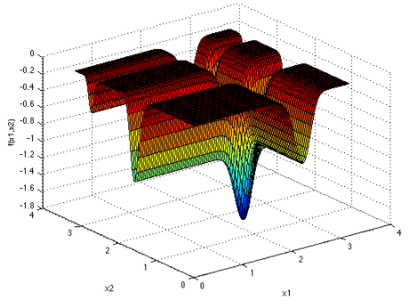
The flower function
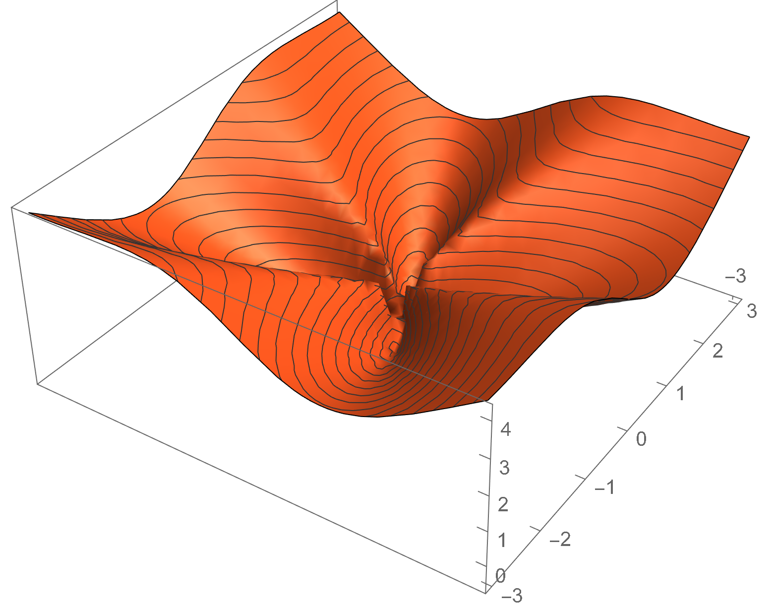
The flower function is the function \(f\colon \R^2 \to \R\) given by
\[f(\vec x) = a \lVert{\vec x}\rVert + b \sin (c \tan^{-1}(x_2, x_1)).\]We use the typical settings of \(a = 1\), \(b = 1\), and \(c = 4\). The function is minimized near origin, although it is undefined at that point.
The Michalewicz function
The \(d\)-dimensional Michalewicz function \(f\colon \mathbb{R}^d \to \mathbb{R}\) is given by
\[f(\vec x) = - \sum_{i=1}^d \sin(x_i)\sin^{2m}\left(\frac{i x_i^2}{\pi}\right).\]It has \(d!\) local minima. Global minima of \(f\) for \(d\) up to 75 are given in [2].
A.3 The CMA-ES algorithm
Algorithm 2: The Covariance Matrix Adaptation Evolutionary Strategy
Require: \(f\colon \R^n \to \R\), initial parameters \((\vec \mu^{(0)}, \vec\Sigma^{(0)}, \sigma^{(0)})\), \(m\) size of sample, \(m_{\text{elite}}\) size of elite subsample.
Ensure: \(\vec \mu^{(T)}\) is the mean of the final distribution and the proposed minimizer.
For \(t = 0, 1, \dotsc\) until convergence:
- Sample points \(\vec x_1, \dotsc, \vec x_m\) from distribution \(N(\vec\mu^{(t)}, \sigma^{(t)}\vec \Sigma^{(t)})\).
- Set \(\vec\mu^{(t+1)}\) according to (\ref{eq:meanstep})
- Set \(\vec\Sigma^{(t+1)}\) according to (\ref{eq:covupdate})
- Set \(\sigma^{(t+1)}\) according to (\ref{eq:stepupdate})
References
[1] Nikolaus Hansen. “The CMA Evolution Strategy: A Tutorial”. In: CoRR abs/1604.00772 (2016). arXiv: 1604.00772. url: http://arxiv.org/abs/1604.00772
[2] Charlie Vanaret et al. “Certified Global Minima for a Benchmark of Difficult Optimization Problems”. In: ArXiv abs/2003.09867 (2020)
[3] S Winter et al. “Registration of CT and Intraoperative 3-D Ultrasound Images of the Spine Using Evolutionary and Gradient-Based Methods”. eng. In: IEEE transactions on evolutionary computation 12.3 (2008), pp. 284–296. issn: 1089-778X.